A quick intro to the ariadne database
Giulio Benedetti
University of Turkugiulio.benedetti@utu.fi
12 May 2026
Source:vignettes/database.Rmd
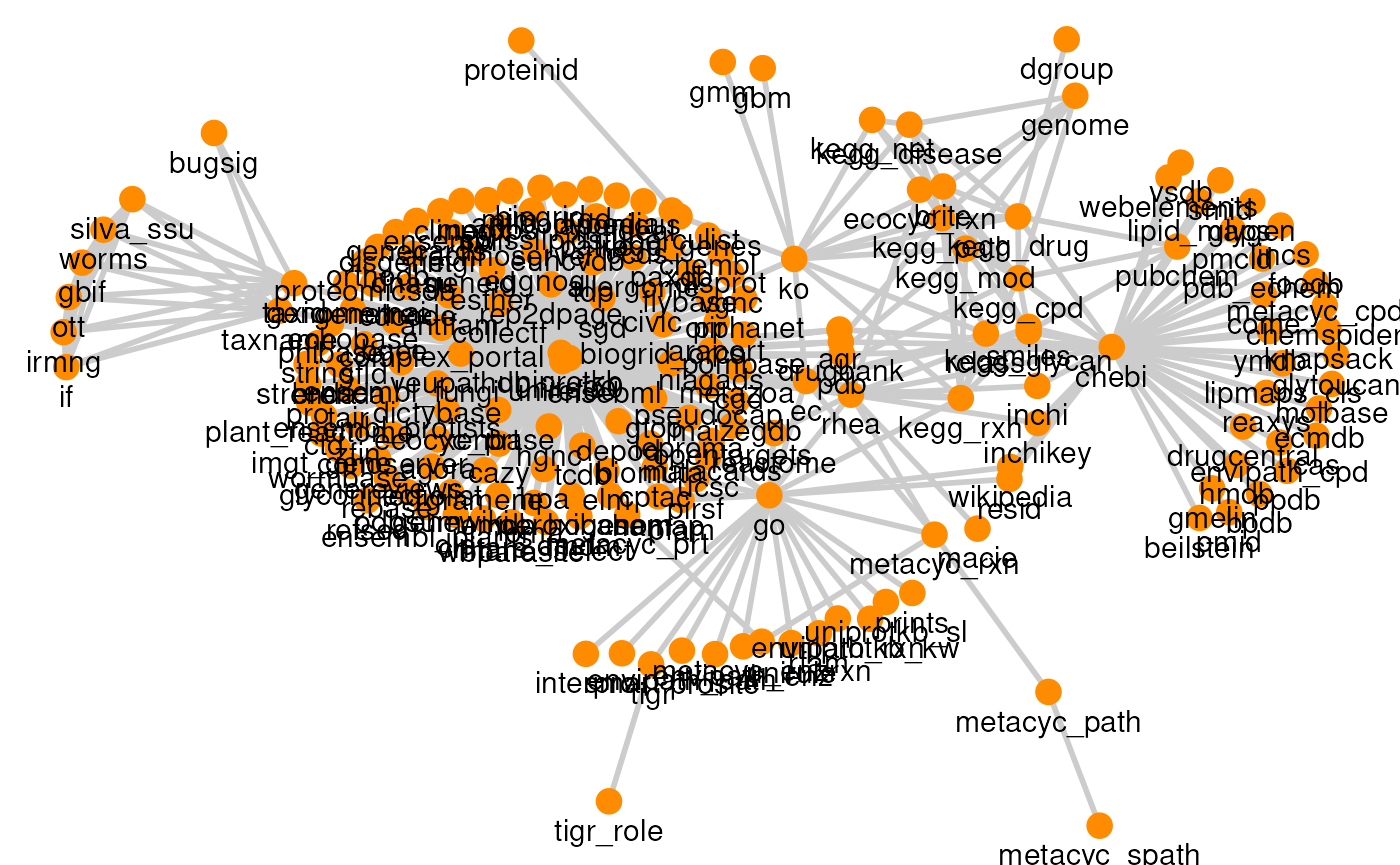
database.RmdThe way that ariadne retrieves and combines relational data is informed by its companion data package ariadne.db, which contains information about the feature types and mappings available from a handful of popular databases. From here on, we will refer to those databases as resources to distinguish them from the ariadne database itself.
The relational information of each resource is described by a graph, where nodes and edges represent feature types and mappings between them, respectively. In ariadne.db, these graphs are stored in the Graph Modelling Language (GML), which is a standard format for relational data.
When ariadne is executed, the graph for each resource is
retrieved from the database release on Zenodo and combined into
a single igraph object.
Some resources have multiple versions, which can be selected through
the argument versions. This defaults to the latest version
found in the database.
# List available resource versions
versions <- listResourceVersions(default = TRUE)

# View versions
knitr::kable(versions)| resource | version | url | |
|---|---|---|---|
| 1 | BugSigDB | v1.3.1 | https://zenodo.org/records/19740674/ |
| 10 | ChocoPhlAn | v201901b | https://zenodo.org/records/17100034/ |
| 16 | GM | v1 | https://github.com/omixer/omixer-rpmR/raw/refs/heads/main/inst/extdata/ |
| 11 | GO | 2026-03-25 | https://release.geneontology.org/2026-03-25/ |
| 18 | KEGG | latest | https://www.genome.jp/kegg/ |
| 19 | OTT | latest | https://opentreeoflife.github.io/ |
| 20 | Rhea | latest | https://www.rhea-db.org/ |
| 17 | TIGRFAMs | v15 | https://ftp.ncbi.nlm.nih.gov/hmm/TIGRFAMs/release_15.0/ |
| 21 | UniProt | latest | https://www.uniprot.org/ |
| 14 | WoL | v2 | https://ftp.microbio.me/pub/wol2/ |
The igraph object is made of two components: edges data and nodes (or vertices) data, which are stored in two different data tables.
# Convert igraph to data.frame pair
graph_df <- igraph::as_data_frame(graph, what = "both")

# Extract edges data
edge_df <- graph_df$edges
# Extract nodes data
node_df <- graph_df$vertices
As mentioned above, the resource graph is composed of feature types (nodes) and mappings (edges) from several resources. Here are the summary statistics for each resource integrated within ariadne:
# Get stats for each resource
df <- edge_df |>
    group_by(source) |>
    summarise(edges = n(), nodes = n_distinct(c(from, to)))

# View stats
knitr::kable(df)| source | edges | nodes |
|---|---|---|
| BugSigDB | 2 | 3 |
| ChocoPhlAn | 11 | 7 |
| GM | 2 | 3 |
| GO | 21 | 22 |
| KEGG | 56 | 20 |
| OTT | 28 | 8 |
| Rhea | 51 | 49 |
| TIGRFAMs | 2 | 3 |
| UniProt | 343 | 117 |
| WoL | 14 | 15 |
The graph for each resource can be visualized with its own graph.
# Create resource graphs
plots <- lapply(df$source, function(x) plotPath(graph, res.name = x))

# View resource graphs
plots
#> [[1]]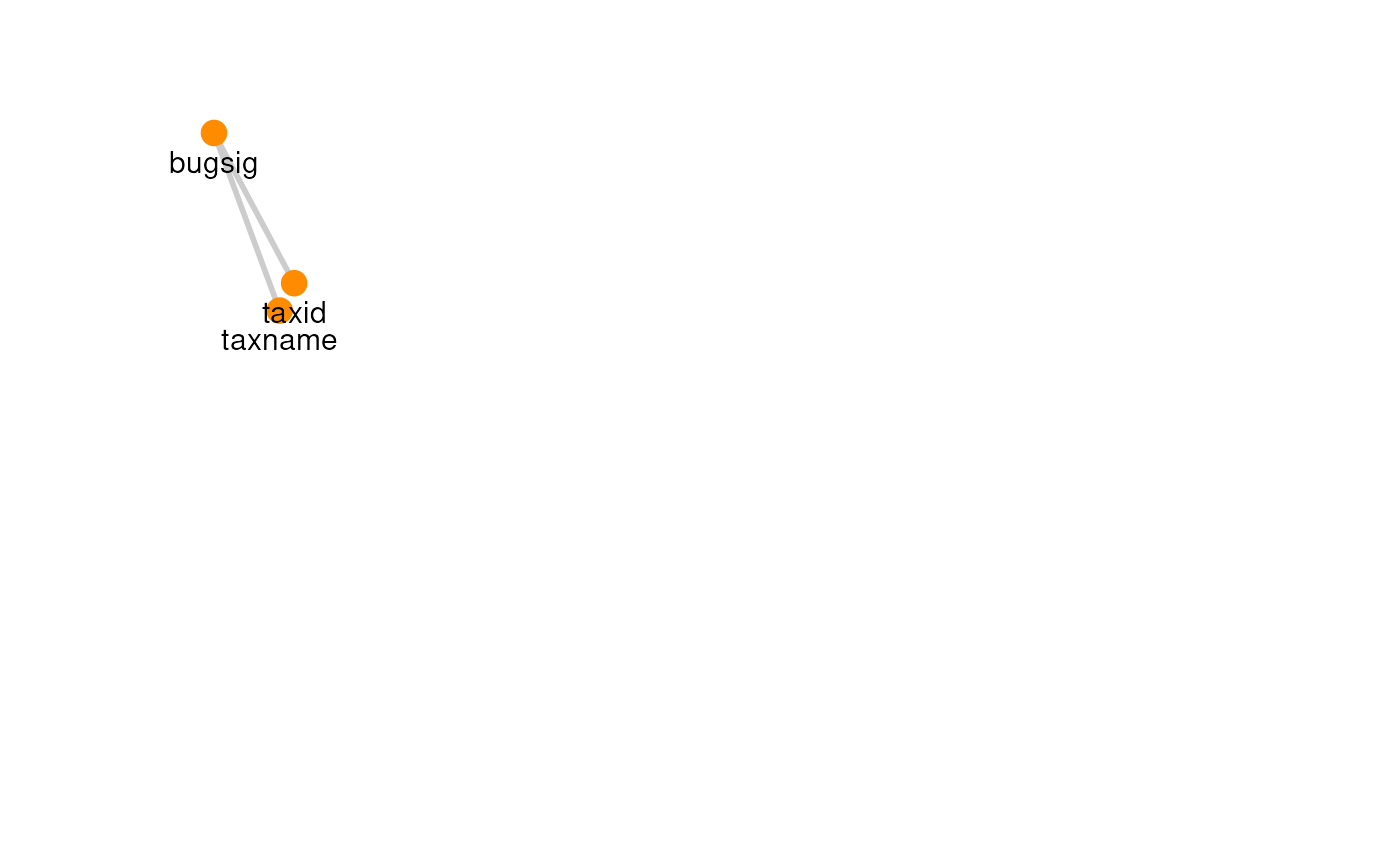
#>
#> [[2]]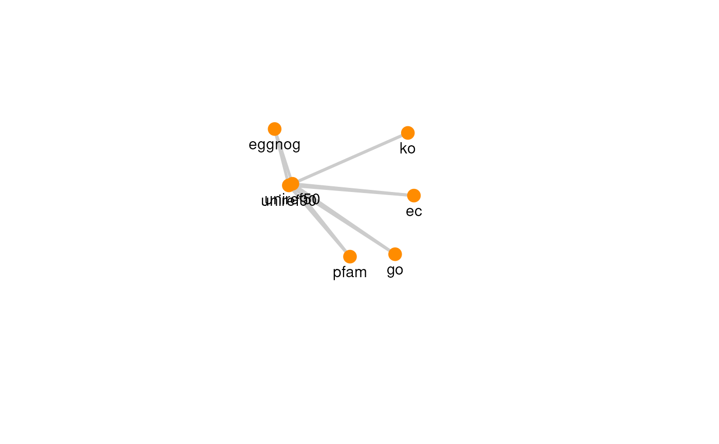
#>
#> [[3]]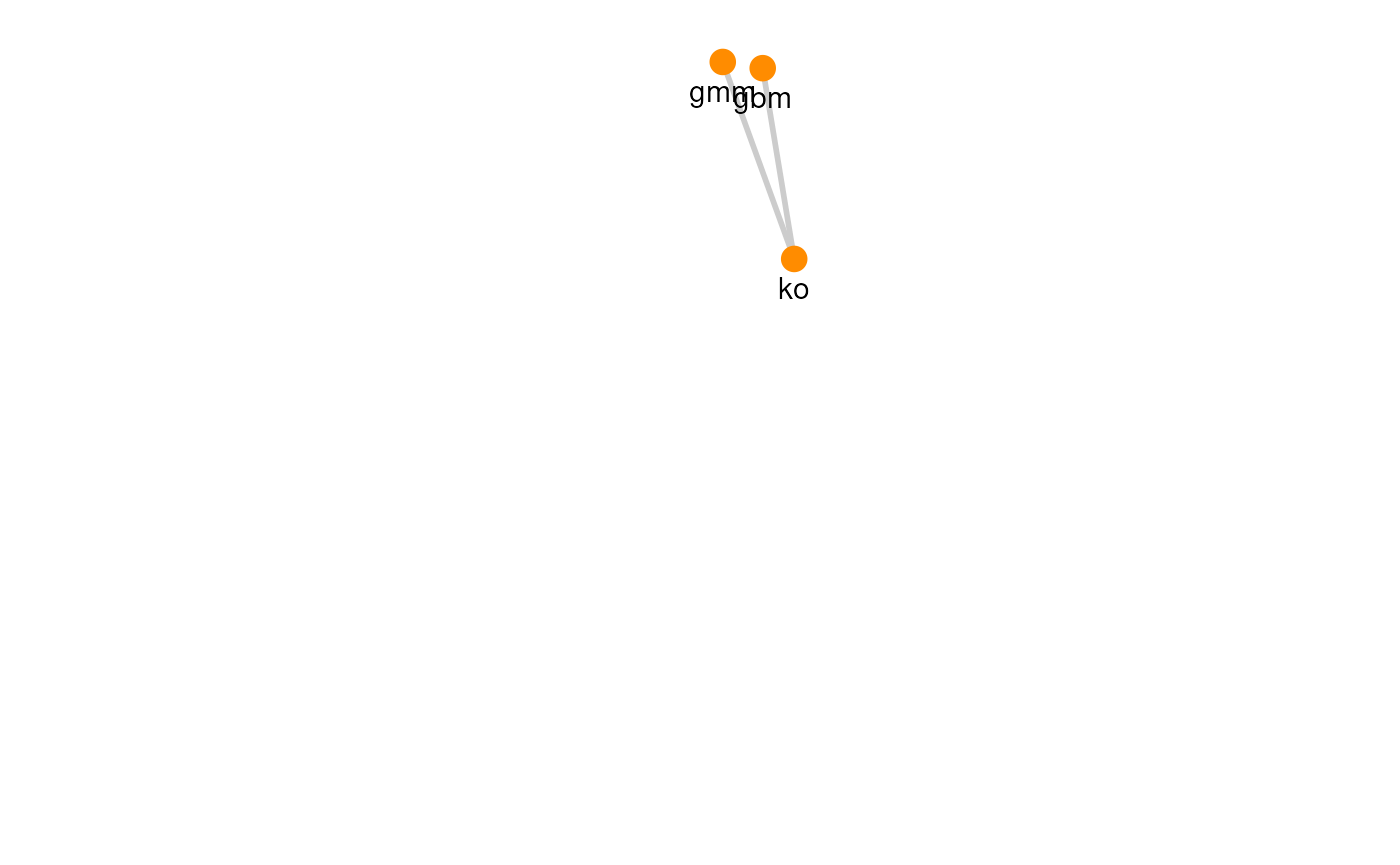
#>
#> [[4]]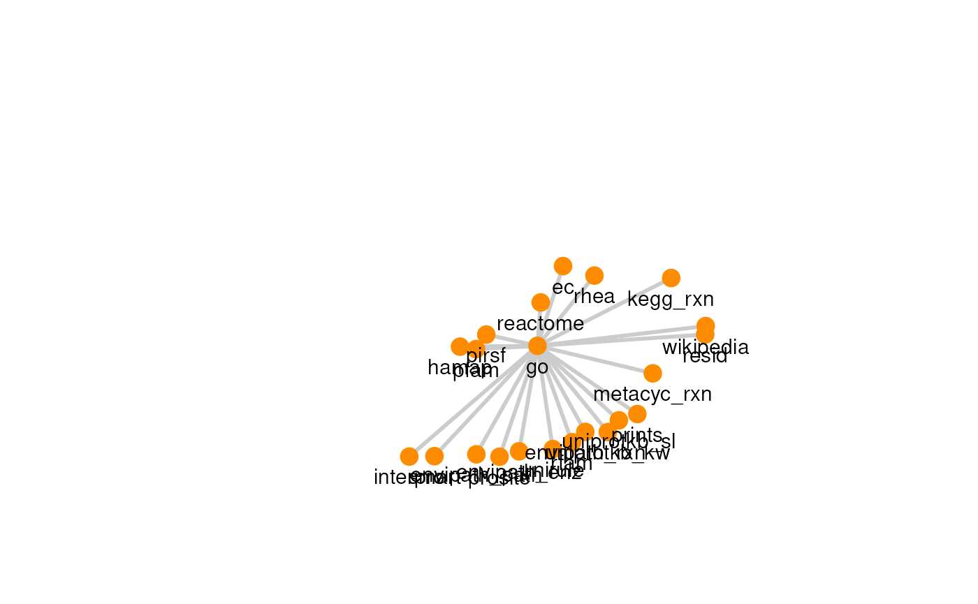
#>
#> [[5]]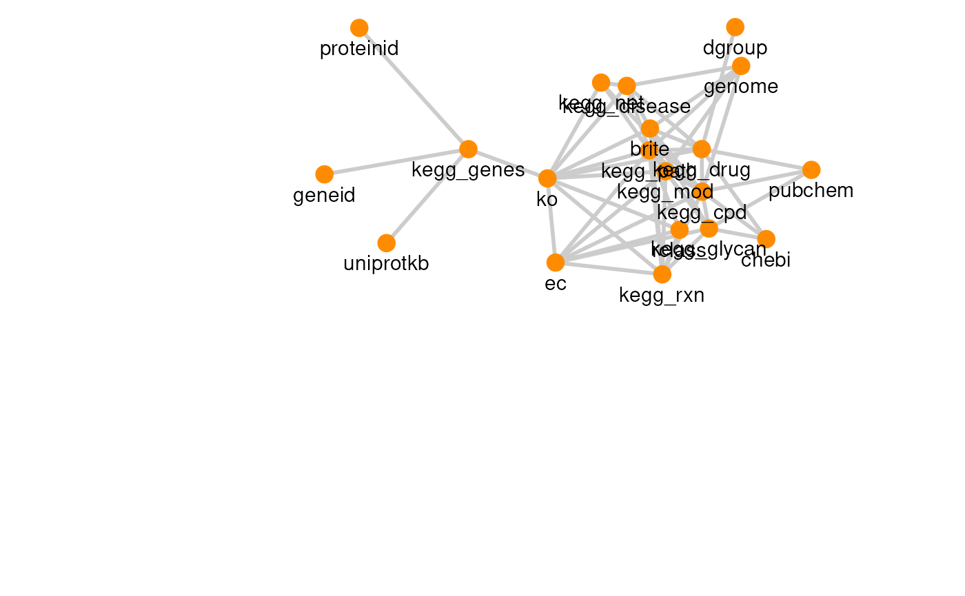
#>
#> [[6]]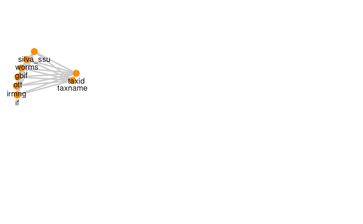
#>
#> [[7]]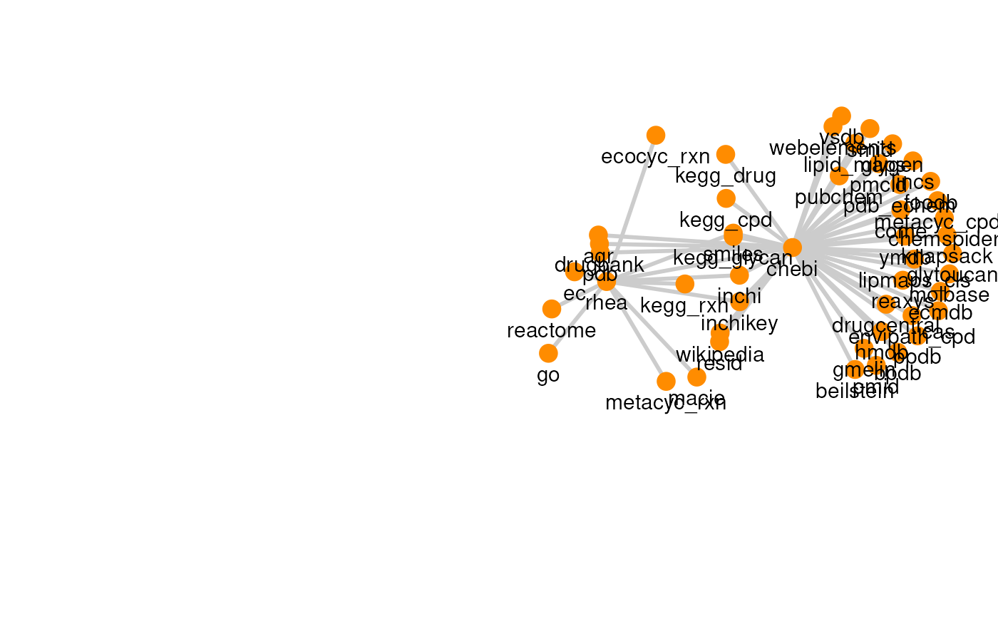
#>
#> [[8]]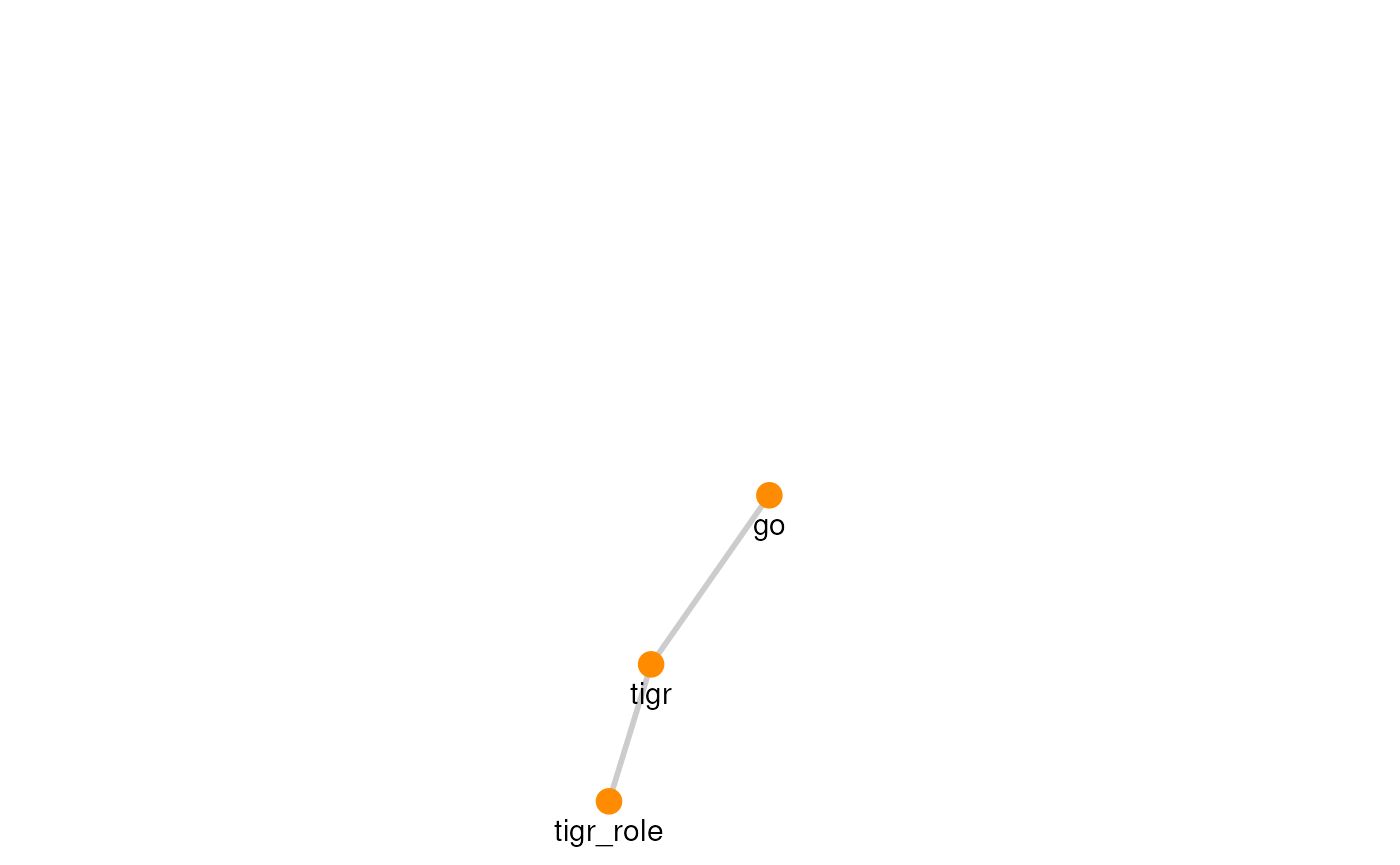
#>
#> [[9]]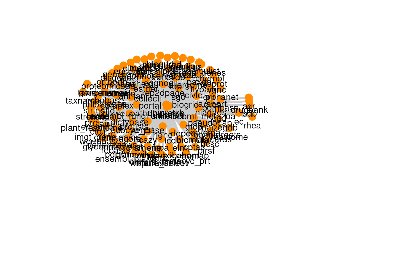
#>
#> [[10]]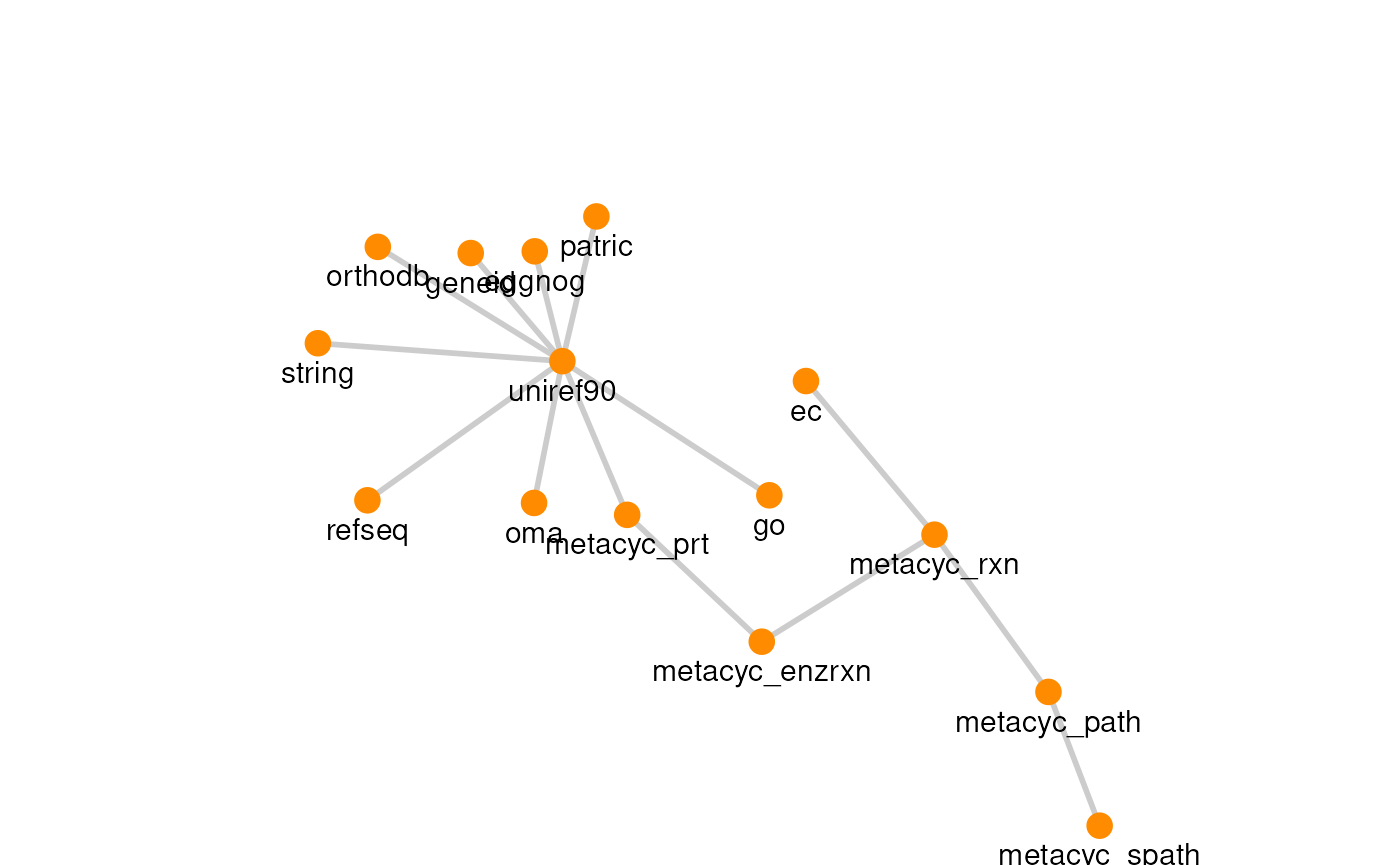
Reproducibility
R session information:
#> R version 4.6.0 (2026-04-24)
#> Platform: x86_64-pc-linux-gnu
#> Running under: Ubuntu 24.04.4 LTS
#>
#> Matrix products: default
#> BLAS:   /usr/lib/x86_64-linux-gnu/openblas-pthread/libblas.so.3
#> LAPACK: /usr/lib/x86_64-linux-gnu/openblas-pthread/libopenblasp-r0.3.26.so;  LAPACK version 3.12.0
#>
#> locale:
#>  [1] LC_CTYPE=en_US.UTF-8       LC_NUMERIC=C               LC_TIME=en_US.UTF-8        LC_COLLATE=en_US.UTF-8
#>  [5] LC_MONETARY=en_US.UTF-8    LC_MESSAGES=en_US.UTF-8    LC_PAPER=en_US.UTF-8       LC_NAME=C
#>  [9] LC_ADDRESS=C               LC_TELEPHONE=C             LC_MEASUREMENT=en_US.UTF-8 LC_IDENTIFICATION=C
#>
#> time zone: UTC
#> tzcode source: system (glibc)
#>
#> attached base packages:
#> [1] stats     graphics  grDevices utils     datasets  methods   base
#>
#> other attached packages:
#> [1] dplyr_1.2.1      igraph_2.3.1     ariadne_0.2.3    BiocStyle_2.41.0
#>
#> loaded via a namespace (and not attached):
#>   [1] DBI_1.3.0                   gridExtra_2.3               httr2_1.2.2                 rlang_1.2.0
#>   [5] magrittr_2.0.5              otel_0.2.0                  matrixStats_1.5.0           compiler_4.6.0
#>   [9] RSQLite_3.52.0              png_0.1-9                   systemfonts_1.3.2           vctrs_0.7.3
#>  [13] stringr_1.6.0               pkgconfig_2.0.3             crayon_1.5.3                fastmap_1.2.0
#>  [17] dbplyr_2.5.2                XVector_0.53.0              labeling_0.4.3              ggraph_2.2.2
#>  [21] rmarkdown_2.31              tzdb_0.5.0                  ragg_1.5.2                  purrr_1.2.2
#>  [25] bit_4.6.0                   xfun_0.57                   cachem_1.1.0                jsonlite_2.0.0
#>  [29] progress_1.2.3              blob_1.3.0                  DelayedArray_0.39.1         BiocParallel_1.47.0
#>  [33] tweenr_2.0.3                prettyunits_1.2.0           parallel_4.6.0              R6_2.6.1
#>  [37] MultiFactor_0.1.2           stringi_1.8.7               bslib_0.10.0                RColorBrewer_1.1-3
#>  [41] GenomicRanges_1.65.0        jquerylib_0.1.4             Rcpp_1.1.1-1.1              Seqinfo_1.3.0
#>  [45] bookdown_0.46               assertthat_0.2.1            SummarizedExperiment_1.43.0 knitr_1.51
#>  [49] readr_2.2.0                 IRanges_2.47.0              rentrez_1.2.4               rotl_3.1.1
#>  [53] Matrix_1.7-5                tidyselect_1.2.1            abind_1.4-8                 yaml_2.3.12
#>  [57] viridis_0.6.5               codetools_0.2-20            curl_7.1.0                  lattice_0.22-9
#>  [61] tibble_3.3.1                Biobase_2.73.1              withr_3.0.2                 KEGGREST_1.53.0
#>  [65] S7_0.2.2                    evaluate_1.0.5              desc_1.4.3                  polyclip_1.10-7
#>  [69] BiocFileCache_3.3.0         Biostrings_2.81.1           pillar_1.11.1               BiocManager_1.30.27
#>  [73] filelock_1.0.3              MatrixGenerics_1.25.0       stats4_4.6.0                generics_0.1.4
#>  [77] S4Vectors_0.51.1            hms_1.1.4                   ggplot2_4.0.3               scales_1.4.0
#>  [81] rncl_0.8.9                  glue_1.8.1                  tools_4.6.0                 data.table_1.18.4
#>  [85] XML_3.99-0.23               fs_2.1.0                    graphlayouts_1.2.3          tidygraph_1.3.1
#>  [89] grid_4.6.0                  ape_5.8-1                   tidyr_1.3.2                 nlme_3.1-169
#>  [93] ggforce_0.5.0               cli_3.6.6                   rappdirs_0.3.4              textshaping_1.0.5
#>  [97] S4Arrays_1.13.0             viridisLite_0.4.3           arrow_24.0.0                gtable_0.3.6
#> [101] sass_0.4.10                 digest_0.6.39               BiocGenerics_0.59.0         SparseArray_1.13.2
#> [105] ggrepel_0.9.8               htmlwidgets_1.6.4           farver_2.1.2                memoise_2.0.1
#> [109] htmltools_0.5.9             pkgdown_2.2.0               lifecycle_1.0.5             httr_1.4.8
#> [113] bit64_4.8.0                 MASS_7.3-65