ariadne: Integrate Knowledge in your Bioinformatic Analysis
Giulio Benedetti
University of Turkugiulio.benedetti@utu.fi
12 May 2026
Source:vignettes/ariadne.Rmd
ariadne.RmdAll domains of biology have to do with relational information. From genes to organisms, each and every biological entity has some link to other entities. For example, bugs are friends or foes with other bugs, have foods they like and foods they hate (sometimes to death). All these links we call relational information, which becomes knowledge once it is smartly combined with other pieces and kept safe and open in a wonderfully organised place, usually a database.
Building a database from scratch is no easy task. Fortunately, nowadays databases for all kinds of relational information are available: UniProt for proteins, Rhea for reactions, KEGG for pretty much anything, and many others, which keep growing together with the field they support. As a scientist, having access to such vast knowledge from past research can truly make us “stand on the shoulders of giants”.
In practice, though, it is not always easy (or even possible) to leverage such knowledge in routine bioinformatic analyses due to three main challenges. First, data is usually deposited somewhere online, so there must be a fast and reliable method to retrieve and import it in the local environment. Second, data size often exceeds the disk space of a typical laptop, which requires smart ways to efficiently subset and store data in a lightweight, accessible format. Third, unless you are lucky, data will need a tidy-up before it is compatible with your dataset and other resources, necessitating a systematic approach to integrate information from multiple resources.
Motivation
Sometimes biology seems like a huge labyrinth with no simple paths between its building blocks (genes, proteins, organisms, etc.). Even when the path to take is clear, many obstacles may hide on the way: inaccessible resources, long query times, incompatible formats, just to name a few. Crossing the labyrinth without a strategy is a seriously boring and discouraging task.
Luckily, ariadne is here to help. By “Assembling Relational Information Across the Database Network”, ariadne provides a harmonised graph of interlinked resources and a rich toolkit to navigate its underexplored paths.
The harmonised graph of resources was built with a reproducible
pipeline hosted in the companion package ariadne.db, and it
is openly available on Zenodo, including its
previous versions.
Implementation
Before describing how ariadne functions, let us explain some important jargon:
-
feature type: a distinct type of biological entity
which includes a set of unique elements labelled with ids. For
consistency, all feature types are written in lower case characters.
Examples:
genes, (KEGG genes id),ko(KEGG Orthologues),ec(Enzyme Commission number) oruniref90(90% similarity UniRef sequence clusters). - level: a unique element belonging to a feature type. The term feature could be used as well, but it is not ideal due to its many closely related meanings. Examples: 563 (NCBI id for E. coli), C00246 (KEGG compound id for butyrate) or P0DTC2 (UniProtKB id for the SARS-CoV-2 spike protein).
-
linkmap: 2-column data.frame where columns are the
feature types and rows the links between them. This is how relational
information is represented in ariadne. It is often named with the syntax
x2y, where x and y are the names of the feature types in the first and second columns, respectively. Sometimes, there is also a third column with the names for the target feature type y. Examples:tax2cpd(linkmap between taxon names and compounds). - resource: a database from where linkmaps between feature types can be retrieved. Examples: KEGG, Rhea or UniProt.
-
weave: the operation of sequentially linking
feature types to generate a new linkmap between two feature types that
originally were not directly linked. This operation follows the syntax
x ~ y, where x and y are the origin and target feature type to be linked, respectively. Examples:ko ~ ec,disease ~ drug,genes ~ metacyc.
Looking inside ariadne:
- The resource graph is represented as an
igraphobject, where edges are resources and nodes feature types. This is a natural choice for relational data and enables applying graph theory to select the preferred path from one feature type to another. It can be also easily expanded with user-defined resources. - Resources are queried via fast
httr2requests or using pre-existing APIs. Whenever possible, even faster SPARQL queries are used to fetch linkmaps. - Linkmaps are automatically cached with
BiocFileCacheand efficiently stored and imported using the Apache parquet columnar format fromarrow. - The
MultiFactorclass, designed for optimised factor operations, takes care of generating the desired linkmap by sequentially weaving linkmaps along the path from the origin to the target feature type.
Applications
ariadne provides a graph-based approach to integrate relational knowledge in routine bioinformatic analyses. As such, it can be used to annotate any type of biological data when related databases are available. This opens up potential applications in various corners of bioinformatics, from knowledge-driven feature annotation and stratification to goal-oriented feature selection and prediction.
With microbes as features, ariadne allows to functionally annotate them using ChocoPhlAn or WoL and to stratify them by Bug Signatures or Gut Modules. (ideas for examples with metabolites, proteins, genes etc?)
ariadne is interoperable with the Bioconductor ecosystem. In particular, the SummarizedExperiment (SE) data container and its derived classes can be directly annotated or stratified by relational information with ariadne.
Tutorial
Installation
if( !requireNamespace("BiocManager", quietly = TRUE) ){
    install.packages("BiocManager")
}

BiocManager::install("ariadne")
Explore the resource graph
ariadne combines different resources into a single graph highlighting
the links between biological entities. The resource graph can be
imported as an igraph object with the function ariadne.
library(ariadne)
library(igraph)

# Import resource graph
graph <- ariadne()

# View graph
summary(graph)
#> IGRAPH dab97b1 DN-- 197 530 --
#> + attr: name (v/c), BugSigDB (v/c), ChocoPhlAn (v/c), GM (v/c), GO
#> | (v/c), KEGG (v/c), OTT (v/c), Rhea (v/c), TIGRFAMs (v/c), UniProt
#> | (v/c), WoL (v/c), url (v/c), source (e/c), url (e/c)
The graph can be explored using all native functions from the igraph package. For example, we can sort its nodes by degree, that is, the number of adjacent edges:
node_degrees <- graph |>
    degree(mode = "all") |>
    sort(decreasing = TRUE)

node_degrees <- node_degrees[node_degrees >= 10]

knitr::kable(node_degrees, col.names = "degree")| degree | |
|---|---|
| uniref90 | 130 |
| uniref50 | 121 |
| uniprotkb | 115 |
| chebi | 44 |
| go | 26 |
| ec | 15 |
| rhea | 15 |
| ko | 14 |
| kegg_cpd | 12 |
| kegg_path | 11 |
| taxid | 11 |
| taxname | 11 |
| kegg_rxn | 10 |
In addition, we can list all the nodes in the neighbourhood of a certain node:
neighbors(graph, "ko", mode = "all")
#> + 14/197 vertices, named, from dab97b1:
#>  [1] brite        ec           gbm          gmm          kegg_disease
#>  [6] kegg_drug    kegg_genes   kegg_mod     kegg_net     kegg_path
#> [11] kegg_rxn     rclass       uniref50     uniref90
The graph can also be visualised with plotPath.
# Plot resource graph
plotPath(graph)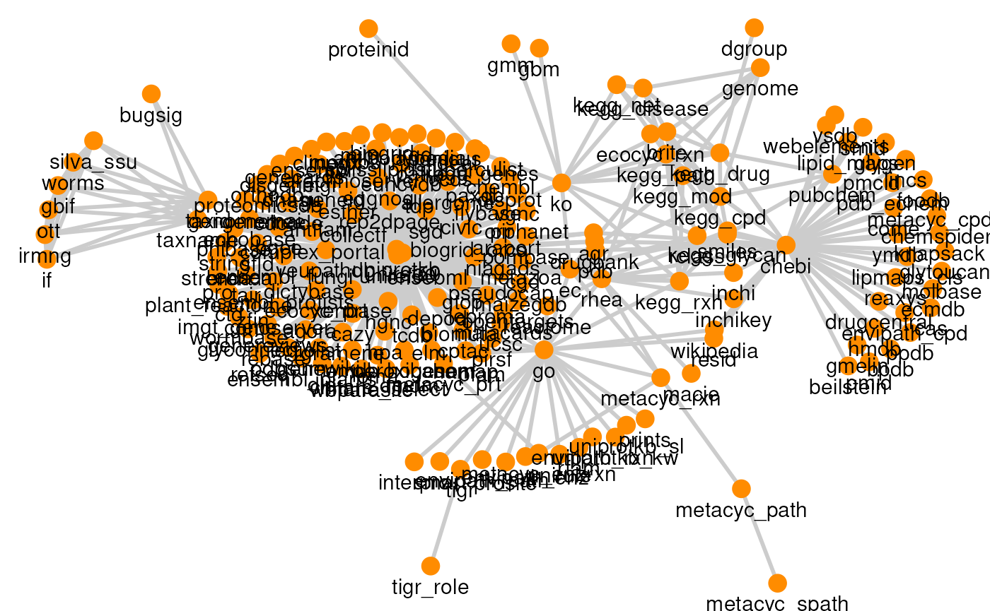
Let’s say we need to find all links between gene functions and enzyme
activity represented by KEGG Orthologues (KO) and Enzyme Commission (EC)
ids, respectively. The function searchPath can be used to
find the k shortest paths in the graph.
# Search for paths from ko to ec
searchPath(graph, ko ~ ec, k = 3)
#> Path 1:
#> ko -(KEGG)-> ec
#>
#> Path 2:
#> ko -(ChocoPhlAn)-> uniref90 -(UniProt)-> ec
#>
#> Path 3:
#> ko -(ChocoPhlAn)-> uniref50 -(UniProt)-> ec
plotPath(graph, ko ~ ec, include = "uniref90", focus = TRUE)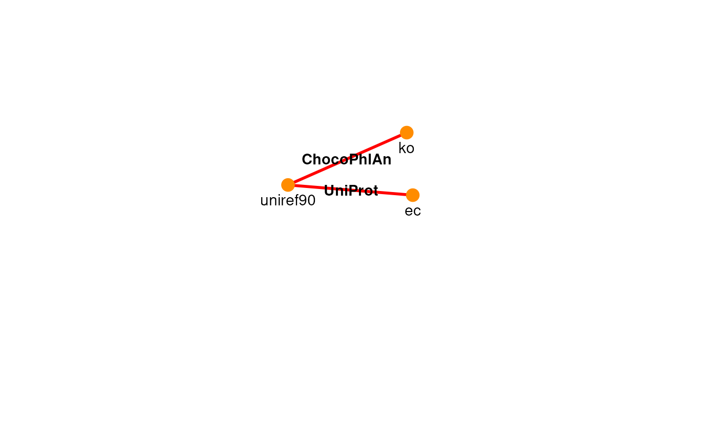
We decide to go through the simplest path, which corresponds to a
k of 1. The links between KO and EC are found by the
function weavePath, which fetches the necessary resources
and weaves a path from KO to EC.
# Weave path from ko to ec
ko2ec <- weavePath(graph, ko ~ ec, k = 1)
#> ko -(KEGG)-> ec
#> Warning: names for 3 ec ids not found.

# View some links
head(ko2ec)
#>       ko      ec               ec.name
#> 1 K00001 1.1.1.1 alcohol dehydrogenase
#> 2 K00121 1.1.1.1 alcohol dehydrogenase
#> 3 K04072 1.1.1.1 alcohol dehydrogenase
#> 4 K11440 1.1.1.1 alcohol dehydrogenase
#> 5 K13951 1.1.1.1 alcohol dehydrogenase
#> 6 K13952 1.1.1.1 alcohol dehydrogenase
The links are provided as a linkmap, a 2-column table where each row is a pair of ids (one KO and one EC). When available, the feature names are returned as a third optional column.
Resources
Citation
We hope that ariadne will be useful for your research. Please use the following information to cite the package and the overall approach. Thank you!
## Citation info
citation("ariadne")
#> Warning in citation("ariadne"): could not determine year for 'ariadne' from
#> package DESCRIPTION file
#> To cite package 'ariadne' in publications use:
#>
#>   Benedetti G, Bastiaanssen T, Lahti L (????). _ariadne: Assembling
#>   Relational Information Across the Database NEtwork_. R package
#>   version 0.2.3, <https://github.com/Minotau-R/ariadne>.
#>
#> A BibTeX entry for LaTeX users is
#>
#>   @Manual{,
#>     title = {ariadne: Assembling Relational Information Across the Database NEtwork},
#>     author = {Giulio Benedetti and Thomaz Bastiaanssen and Leo Lahti},
#>     note = {R package version 0.2.3},
#>     url = {https://github.com/Minotau-R/ariadne},
#>   }
Background Knowledge
ariadne originates from the joint effort of the R/Bioconductor community. It is mainly based on the following software:
- R, statistical programming language [@core2025r]
- mia, framework for microbiome data analysis [@borman2025mia]
- MultiFactor, Annotation-based Analysis of Specific Interactions [@bastiaanssen2023anansi]
- TreeSummarizedExperiment, S4 container for hierarchical data [@huang2020treesummarizedexperiment]
Help
You can reach us by one of the communication channels listed here. We are happy to receive questions, suggestions as well as contributions. For the last point, check the contributor guidelines.
Reproducibility
R session information:
#> R version 4.6.0 (2026-04-24)
#> Platform: x86_64-pc-linux-gnu
#> Running under: Ubuntu 24.04.4 LTS
#>
#> Matrix products: default
#> BLAS:   /usr/lib/x86_64-linux-gnu/openblas-pthread/libblas.so.3
#> LAPACK: /usr/lib/x86_64-linux-gnu/openblas-pthread/libopenblasp-r0.3.26.so;  LAPACK version 3.12.0
#>
#> locale:
#>  [1] LC_CTYPE=en_US.UTF-8       LC_NUMERIC=C               LC_TIME=en_US.UTF-8        LC_COLLATE=en_US.UTF-8
#>  [5] LC_MONETARY=en_US.UTF-8    LC_MESSAGES=en_US.UTF-8    LC_PAPER=en_US.UTF-8       LC_NAME=C
#>  [9] LC_ADDRESS=C               LC_TELEPHONE=C             LC_MEASUREMENT=en_US.UTF-8 LC_IDENTIFICATION=C
#>
#> time zone: UTC
#> tzcode source: system (glibc)
#>
#> attached base packages:
#> [1] stats     graphics  grDevices utils     datasets  methods   base
#>
#> other attached packages:
#> [1] igraph_2.3.1     ariadne_0.2.3    BiocStyle_2.41.0
#>
#> loaded via a namespace (and not attached):
#>   [1] DBI_1.3.0                   gridExtra_2.3               httr2_1.2.2                 rlang_1.2.0
#>   [5] magrittr_2.0.5              otel_0.2.0                  matrixStats_1.5.0           compiler_4.6.0
#>   [9] RSQLite_3.52.0              png_0.1-9                   systemfonts_1.3.2           vctrs_0.7.3
#>  [13] stringr_1.6.0               pkgconfig_2.0.3             crayon_1.5.3                fastmap_1.2.0
#>  [17] dbplyr_2.5.2                XVector_0.53.0              labeling_0.4.3              ggraph_2.2.2
#>  [21] rmarkdown_2.31              tzdb_0.5.0                  ragg_1.5.2                  purrr_1.2.2
#>  [25] bit_4.6.0                   xfun_0.57                   cachem_1.1.0                jsonlite_2.0.0
#>  [29] progress_1.2.3              blob_1.3.0                  DelayedArray_0.39.1         BiocParallel_1.47.0
#>  [33] tweenr_2.0.3                prettyunits_1.2.0           parallel_4.6.0              R6_2.6.1
#>  [37] MultiFactor_0.1.2           stringi_1.8.7               bslib_0.10.0                RColorBrewer_1.1-3
#>  [41] GenomicRanges_1.65.0        jquerylib_0.1.4             Rcpp_1.1.1-1.1              Seqinfo_1.3.0
#>  [45] bookdown_0.46               assertthat_0.2.1            SummarizedExperiment_1.43.0 knitr_1.51
#>  [49] readr_2.2.0                 IRanges_2.47.0              rentrez_1.2.4               rotl_3.1.1
#>  [53] Matrix_1.7-5                tidyselect_1.2.1            abind_1.4-8                 yaml_2.3.12
#>  [57] viridis_0.6.5               codetools_0.2-20            curl_7.1.0                  lattice_0.22-9
#>  [61] tibble_3.3.1                Biobase_2.73.1              withr_3.0.2                 KEGGREST_1.53.0
#>  [65] S7_0.2.2                    evaluate_1.0.5              desc_1.4.3                  polyclip_1.10-7
#>  [69] BiocFileCache_3.3.0         Biostrings_2.81.1           pillar_1.11.1               BiocManager_1.30.27
#>  [73] filelock_1.0.3              MatrixGenerics_1.25.0       stats4_4.6.0                generics_0.1.4
#>  [77] S4Vectors_0.51.1            hms_1.1.4                   ggplot2_4.0.3               scales_1.4.0
#>  [81] rncl_0.8.9                  glue_1.8.1                  tools_4.6.0                 data.table_1.18.4
#>  [85] XML_3.99-0.23               fs_2.1.0                    graphlayouts_1.2.3          tidygraph_1.3.1
#>  [89] grid_4.6.0                  ape_5.8-1                   tidyr_1.3.2                 nlme_3.1-169
#>  [93] ggforce_0.5.0               cli_3.6.6                   rappdirs_0.3.4              textshaping_1.0.5
#>  [97] S4Arrays_1.13.0             viridisLite_0.4.3           arrow_24.0.0                dplyr_1.2.1
#> [101] gtable_0.3.6                sass_0.4.10                 digest_0.6.39               BiocGenerics_0.59.0
#> [105] SparseArray_1.13.2          ggrepel_0.9.8               htmlwidgets_1.6.4           farver_2.1.2
#> [109] memoise_2.0.1               htmltools_0.5.9             pkgdown_2.2.0               lifecycle_1.0.5
#> [113] httr_1.4.8                  bit64_4.8.0                 MASS_7.3-65