MultiFactor
MultiFactor.RmdOverview
MultiFactor aims to provide a consistent toolkit to
incorporate relational data into data-analytical tools and methods. In
practice, we expect MultiFactor to be used in combination
with additional packages that extend it. For instance, see ariadne and anansi, two such
packages that make use of MultiFactor to link and convert
across biological database IDs and perform multi-omics integration
analysis, respectively.
Get started using MultiFactor
Installation instructions
Get the latest stable R release from CRAN. Then install the released
version of MultiFactor:
install.packages("MultiFactor")Or install the development version from this repository:
install.packages("remotes")
remotes::install_github("minotau-R/MultiFactor")
Setup
library(MultiFactor)

# Wrangling
library(dplyr)

# Plotting
library(ggplot2)
library(systemfonts)
library(ragg)

# Load demo data
set.seed(2612)
tp <- trade_posts()
MultiFactor and LinkMap objects
LinkMap
The basic object in the MultiFactor package is the
LinkMap, which contains relational information across two
types of features. This format is sometimes referred to as an edge list. Under a
thin layer of S7, the LinkMap object is a
data.frame where the first two columns indicate which
feature IDs that are considered linked. Optional additional columns are
considered metadata.
Let’s use an example data set to take a closer look at
LinkMap. The trade_posts() function generates
data about fictional trade posts, where one type of good is traded for
another. In this particular case, types of books are traded for types of
furniture.
linkmap <- tp[[1]]
linkmap
#> A MultiFactor::LinkMap data.frame S7_object: 9 rows.
#>        books furniture
#> 1   red book     couch
#> 2 green book   cabinet
#> 3 plain book   cabinet
#> 4  blue book  wastebin
#> 5 plain book  wastebin
#> 6  blue book       box
#> 7 plain book       box
#> 8 fancy book      door
#> 9  blue book      door
#>
#> @ levels:   2 variables:
#>  $ books     : 6 Levels: fancy book ... plain book
#>  $ furniture : 6 Levels: couch ... door
#>
#> @ metadata: 4 variables:
#> List of 4
#>  $ books_emoji    : chr  "📕" "📗" "📓" "📘" ...
#>  $ books_runes    : chr  "1F4D5" "1F4D7" "1F4D3" "1F4D8" ...
#>  $ furniture_emoji: chr  "🛋" "🗄" "🗄" "🗑" ...
#>  $ furniture_runes: chr  "1F6CB" "1F5C4" "1F5C4" "1F5D1" ...
The two types of goods are captured by the two columns, with column
names representing the types of good and rows representing
which specific type-pairs are traded at that trade post, or,
more generally, are linked in that LinkMap.
levels( linkmap )
#> $books
#> [1] "fancy book"  "green book"  "red book"    "blue book"   "orange book"
#> [6] "plain book"
#>
#> $furniture
#> [1] "couch"    "cabinet"  "wastebin" "bed"      "box"      "door"
Notice that LinkMap is two factor columns
in a trench coat. We can inspect the levels as usual.
We can see that we have several of these types of trade posts in our data set. However, we also notice that the column names - the types of goods - can differ.
tp[[2]]
#> A MultiFactor::LinkMap data.frame S7_object: 9 rows.
#>   clothing furniture
#> 1    scarf     couch
#> 2    scarf   cabinet
#> 3   gloves  wastebin
#> 4      hat  wastebin
#> 5    scarf  wastebin
#> 6    dress       bed
#> 7  t-shirt       box
#> 8    scarf       box
#> 9      hat      door
#>
#> @ levels:   2 variables:
#>  $ clothing  : 6 Levels: t-shirt ... scarf
#>  $ furniture : 6 Levels: couch ... door
#>
#> @ metadata: 4 variables:
#> List of 4
#>  $ clothing_emoji : chr  "🧣" "🧣" "🧤" "🎩" ...
#>  $ clothing_runes : chr  "1F9E3" "1F9E3" "1F9E4" "1F3A9" ...
#>  $ furniture_emoji: chr  "🛋" "🗄" "🗑" "🗑" ...
#>  $ furniture_runes: chr  "1F6CB" "1F5C4" "1F5D1" "1F5D1" ...
tp[[3]]
#> A MultiFactor::LinkMap data.frame S7_object: 9 rows.
#>         books instruments
#> 1  green book     trumpet
#> 2    red book      guitar
#> 3   blue book      guitar
#> 4   blue book        drum
#> 5  green book    keyboard
#> 6 orange book    keyboard
#> 7    red book      fiddle
#> 8 orange book   saxophone
#> 9  plain book   saxophone
#>
#> @ levels:   2 variables:
#>  $ books       : 6 Levels: fancy book ... plain book
#>  $ instruments : 6 Levels: trumpet ... saxophone
#>
#> @ metadata: 4 variables:
#> List of 4
#>  $ books_emoji      : chr  "📗" "📕" "📘" "📘" ...
#>  $ books_runes      : chr  "1F4D7" "1F4D5" "1F4D8" "1F4D8" ...
#>  $ instruments_emoji: chr  "🎺" "🎸" "🎸" "🥁" ...
#>  $ instruments_runes: chr  "1F3BA" "1F3B8" "1F3B8" "1F941" ...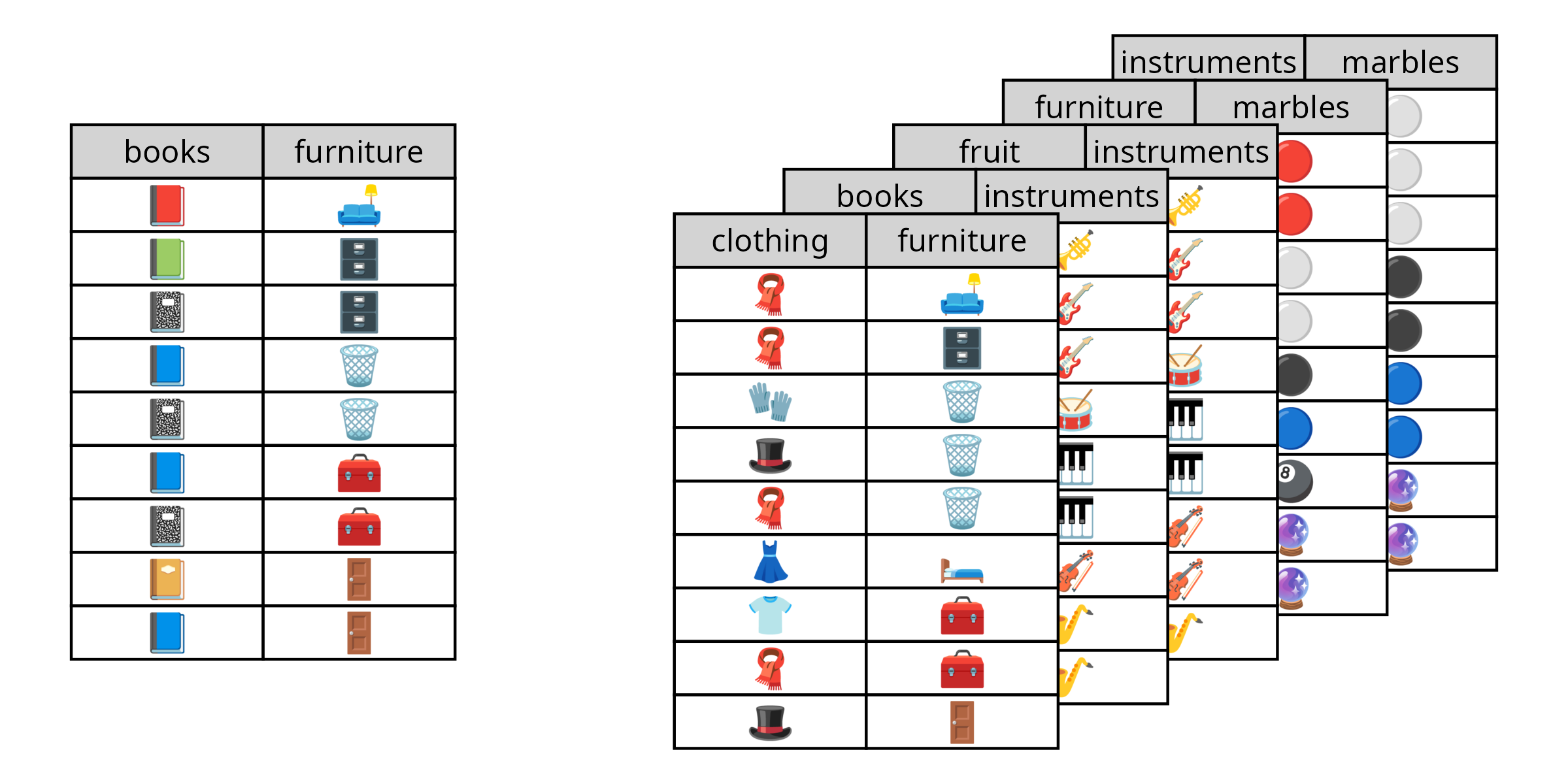
MultiFactor
The MultiFactor is in essence a collection of
LinkMaps. Where LinkMaps contain relational
information across two data types, MultiFactors are a
representation of the relational graph formed by combining those
LinkMaps. The full object tp, which contains
the LinkMaps we just investigated, is in fact a
MultiFactor object:
tp
#> A MultiFactor::MultiFactor list S7_object,
#>     6 feature types across 6 LinkMaps.
#>
#>                     books furniture clothing instruments fruit marbles
#> books2furniture         5         5        .           .     .       .
#> clothing2furniture      .         6        5           .     .       .
#> books2instruments       5         .        .           6     .       .
#> fruit2instruments       .         .        .           6     5       .
#> furniture2marbles       .         5        .           .     .       6
#> instruments2marbles     .         .        .           5     .       4
#>
#> Values represent unique feature names in that LinkMap.
#>
#> @ levels:
#>  $ books       : 6 Levels: fancy book ... plain book
#>  $ furniture   : 6 Levels: couch ... door
#>  $ clothing    : 6 Levels: t-shirt ... scarf
#>  $ instruments : 6 Levels: trumpet ... saxophone
#>  $ fruit       : 6 Levels: apples ... grapes
#>  $ marbles     : 6 Levels: red marble ... sparkly marble
Notice that a MultiFactor summarizes information across
the component LinkMaps in several ways. First, The matrix
shows the types of goods as columns and the component
LinkMaps that contain this information as rows. The numbers
in the matrix then show the number of unique types of that type of good
in that particular LinkMap - and that are therefore linked
to the second feature in the LinkMap.
For instance, in the top-left corner of the matrix, we can see that
the first LinkMap links books and furniture and is aptly
named books2furniture. Notice that five unique types of
books as well as five types of furniture are mentioned in
books2furniture.
Though MultiFactor is a list of LinkMaps
under the hood, we can also interact with its matrix representation, as
well as access the component levels:
dim(tp)
#> [1] 6 6
dimnames(tp)
#> [[1]]
#> [1] "books2furniture"     "clothing2furniture"  "books2instruments"
#> [4] "fruit2instruments"   "furniture2marbles"   "instruments2marbles"
#>
#> [[2]]
#> [1] "books"       "furniture"   "clothing"    "instruments" "fruit"
#> [6] "marbles"
levels(tp)
#> $books
#> [1] "fancy book"  "green book"  "red book"    "blue book"   "orange book"
#> [6] "plain book"
#>
#> $clothing
#> [1] "t-shirt" "dress"   "socks"   "gloves"  "hat"     "scarf"
#>
#> $fruit
#> [1] "apples"   "pears"    "cherries" "oranges"  "melons"   "grapes"
#>
#> $furniture
#> [1] "couch"    "cabinet"  "wastebin" "bed"      "box"      "door"
#>
#> $instruments
#> [1] "trumpet"   "guitar"    "drum"      "keyboard"  "fiddle"    "saxophone"
#>
#> $marbles
#> [1] "red marble"     "white marble"   "black marble"   "blue marble"
#> [5] "8 marble"       "sparkly marble"
nlevels(tp)
#>       books    clothing       fruit   furniture instruments     marbles
#>           6           6           6           6           6           6
Note that levels of the same type are automatically unified across all component LinkMaps with that type of level.
weave() a path
Going back to our trading post example, let’s say we’d want to get
some new hats, but we only have fruit. While both fruit and clothing are
available in our data set, there aren’t any trade post that deals in
that particular pair of goods. However, we could imagine trading our
fruit for clothing in steps: We can trade our fruit for a different
good, which we trade for another one, until we reach a good that we can
trade for clothing. The weave() function does exactly
this:
fruit2clothing <- weave(tp, fruit ~ clothing)
fruit2clothing
#> A MultiFactor::LinkMap data.frame S7_object: 18 rows.
#>      fruit clothing
#> 1   apples  t-shirt
#> 2    pears  t-shirt
#> 3   apples   gloves
#> 4    pears   gloves
#> 5   apples      hat
#> 6    pears      hat
#> 7   apples    scarf
#> 8    pears    scarf
#> 9  oranges    scarf
#> 10  melons    scarf
#>  + 8 more rows. Use `print(n = ...)` to see more rows.
#>
#> @ levels:   2 variables:
#>  $ fruit    : 6 Levels: apples ... grapes
#>  $ clothing : 6 Levels: t-shirt ... scarf
We receive a new LinkMap containing all fruits that
could be traded for clothing.
Selecting a path
We can use select_path() to find the types of traded
goods in order, or more generally, the paths that were traversed. If
several paths exist, all will be traversed and included into one
LinkMap.
select_path(tp, fruit ~ clothing)
#> A MultiFactor::factor_path S7_object from `fruit` to `clothing` with 2 sub-paths:
#> [[1]]
#> [1] "fruit"       "instruments" "books"       "furniture"   "clothing"
#>
#> [[2]]
#> [1] "fruit"       "instruments" "marbles"     "furniture"   "clothing"
Compatibility with igraph and Matrix
Convert MultiFactor and LinkMap objects to
igraph representation
MultiFactor relies heavily on the excellent igraph and Matrix
packages, particularly for path finding and sparse matrix
representation.
Convert MultiFactor main graph representation to
igraph object
library(igraph)
#>
#> Attaching package: 'igraph'
#> The following objects are masked from 'package:dplyr':
#>
#>     as_data_frame, groups, union
#> The following objects are masked from 'package:stats':
#>
#>     decompose, spectrum
#> The following object is masked from 'package:base':
#>
#>     union
# Convert to an igraph object
g <- as.igraph(tp)
g
#> IGRAPH 280c1f0 UN-- 6 6 --
#> + attr: name (v/c), name (e/c), instruments_emoji (e/n),
#> | instruments_runes (e/n), marbles_emoji (e/n), marbles_runes (e/n),
#> | furniture_emoji (e/n), furniture_runes (e/n), books_emoji (e/n),
#> | books_runes (e/n), clothing_emoji (e/n), clothing_runes (e/n),
#> | fruit_emoji (e/n), fruit_runes (e/n)
#> + edges from 280c1f0 (vertex names):
#> [1] books      --furniture   clothing   --furniture   books      --instruments
#> [4] fruit      --instruments furniture  --marbles     instruments--marbles
# Plot graph across data types
plot(g)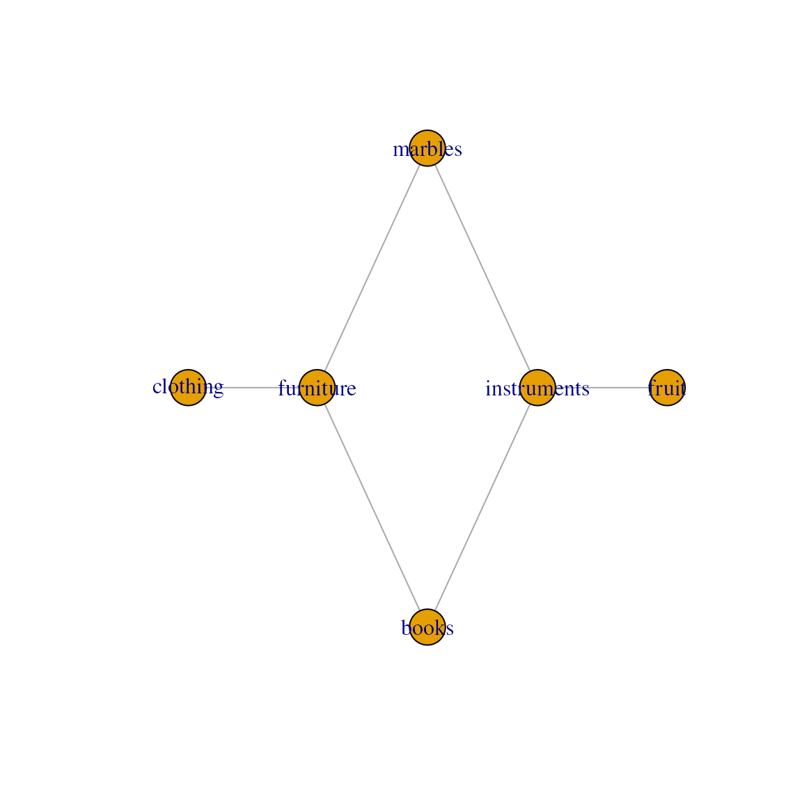
Convert LinkMap relational information to
igraph object
# Convert to an igraph object
lg <- as.igraph(fruit2clothing)
lg
#> IGRAPH e39809f UN-B 12 18 --
#> + attr: type (v/l), name (v/c)
#> + edges from e39809f (vertex names):
#>  [1] apples --t-shirt pears  --t-shirt apples --dress   oranges--dress
#>  [5] melons --dress   grapes --dress   apples --gloves  pears  --gloves
#>  [9] apples --hat     pears  --hat     oranges--hat     melons --hat
#> [13] grapes --hat     apples --scarf   pears  --scarf   oranges--scarf
#> [17] melons --scarf   grapes --scarf
# Same information as the LinkMap:
plot(lg)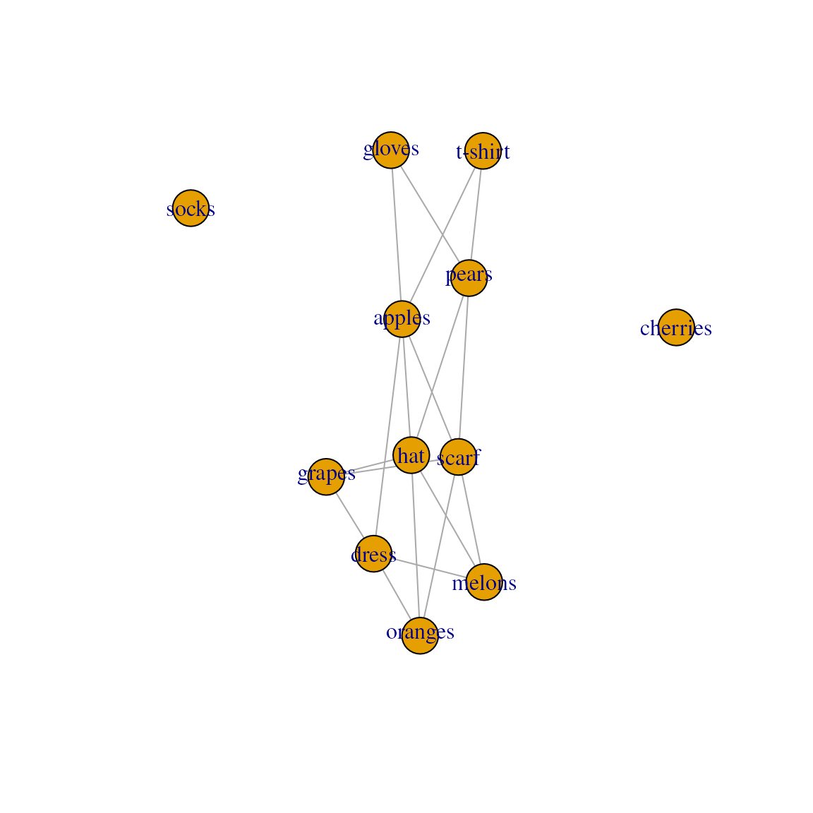
Convert LinkMap linkage information to sparse adjacency
Matrix
# Convert to an igraph object
m <- as.matrix(fruit2clothing)
m
#> 6 x 6 sparse Matrix of class "ngCMatrix"
#>           clothing
#> fruit      t-shirt dress socks gloves hat scarf
#>   apples         |     |     .      |   |     |
#>   pears          |     .     .      |   |     |
#>   cherries       .     .     .      .   .     .
#>   oranges        .     |     .      .   |     |
#>   melons         .     |     .      .   |     |
#>   grapes         .     |     .      .   |     |
Utilities
MultiFactor also provides some utility functions for
data wrangling on tables with features (rows) of the appropriate
type.
# Generate small example table
generate_sample <- function(n) rbinom(n, rbinom(n, 100, runif(n)), runif(n))
n <- nlevels(tp)[["clothing"]]

clothing_table <- as.data.frame( replicate( 10,  generate_sample(n)) )
rownames(clothing_table) <- levels(tp)$clothing

clothing_table
#>         V1 V2 V3 V4 V5 V6 V7 V8 V9 V10
#> t-shirt 14  8 34 72 47  4 32 50  0   5
#> dress   16 11 34 40 35 63  2 28  0  42
#> socks   20 24 20 50  2  0 19  5 17  46
#> gloves   0 34 10  2 21 30  0  3 13  16
#> hat      0 61  0  4  3  0  7 20 38  21
#> scarf    4 80 47 72 29 55  4  4 16  25
weave_apply
weave_apply allows us to run arbitrary code on subsets
of a table, based on groupings on the left hand of the formula:
weave_apply(
  .x = tp, .path = fruit ~ clothing,
  .data = clothing_table, .fun = as.data.frame
  )
#> $apples
#>         V1 V2 V3 V4 V5 V6 V7 V8 V9 V10
#> dress   16 11 34 40 35 63  2 28  0  42
#> hat      0 61  0  4  3  0  7 20 38  21
#> scarf    4 80 47 72 29 55  4  4 16  25
#> t-shirt 14  8 34 72 47  4 32 50  0   5
#> gloves   0 34 10  2 21 30  0  3 13  16
#>
#> $pears
#>         V1 V2 V3 V4 V5 V6 V7 V8 V9 V10
#> t-shirt 14  8 34 72 47  4 32 50  0   5
#> gloves   0 34 10  2 21 30  0  3 13  16
#> hat      0 61  0  4  3  0  7 20 38  21
#> scarf    4 80 47 72 29 55  4  4 16  25
#>
#> $oranges
#>       V1 V2 V3 V4 V5 V6 V7 V8 V9 V10
#> dress 16 11 34 40 35 63  2 28  0  42
#> hat    0 61  0  4  3  0  7 20 38  21
#> scarf  4 80 47 72 29 55  4  4 16  25
#>
#> $melons
#>       V1 V2 V3 V4 V5 V6 V7 V8 V9 V10
#> dress 16 11 34 40 35 63  2 28  0  42
#> hat    0 61  0  4  3  0  7 20 38  21
#> scarf  4 80 47 72 29 55  4  4 16  25
#>
#> $grapes
#>       V1 V2 V3 V4 V5 V6 V7 V8 V9 V10
#> dress 16 11 34 40 35 63  2 28  0  42
#> hat    0 61  0  4  3  0  7 20 38  21
#> scarf  4 80 47 72 29 55  4  4 16  25

# More complex example:
# For all subgroups of clothing corresponding to one particular fruit, if that
# group has more than two rows (types of clothing), fit a statistical model.
#
weave_apply(
  tp, fruit ~ clothing, clothing_table, function(x) {
    if( NROW(x) <= 2 ) return( NULL )
    # else:
    summary( lm(V1 ~ V2, data = x) )
    }
)
#> $apples
#>
#> Call:
#> lm(formula = V1 ~ V2, data = x)
#>
#> Residuals:
#>   dress     hat   scarf t-shirt  gloves
#>   4.175  -2.787   4.647   1.633  -7.668
#>
#> Coefficients:
#>             Estimate Std. Error t value Pr(>|t|)
#> (Intercept) 13.81295    4.58505   3.013   0.0571 .
#> V2          -0.18075    0.09576  -1.887   0.1555
#> ---
#> Signif. codes:  0 '***' 0.001 '**' 0.01 '*' 0.05 '.' 0.1 ' ' 1
#>
#> Residual standard error: 6.007 on 3 degrees of freedom
#> Multiple R-squared:  0.5428, Adjusted R-squared:  0.3905
#> F-statistic: 3.562 on 1 and 3 DF,  p-value: 0.1555
#>
#>
#> $pears
#>
#> Call:
#> lm(formula = V1 ~ V2, data = x)
#>
#> Residuals:
#> t-shirt  gloves     hat   scarf
#>   4.522  -6.050  -2.489   4.017
#>
#> Coefficients:
#>             Estimate Std. Error t value Pr(>|t|)
#> (Intercept)  10.5332     6.1564   1.711    0.229
#> V2           -0.1319     0.1156  -1.141    0.372
#>
#> Residual standard error: 6.3 on 2 degrees of freedom
#> Multiple R-squared:  0.3941, Adjusted R-squared:  0.09117
#> F-statistic: 1.301 on 1 and 2 DF,  p-value: 0.3722
#>
#>
#> $oranges
#>
#> Call:
#> lm(formula = V1 ~ V2, data = x)
#>
#> Residuals:
#>  dress    hat  scarf
#>  1.256 -4.563  3.306
#>
#> Coefficients:
#>             Estimate Std. Error t value Pr(>|t|)
#> (Intercept)  16.9835     6.6920   2.538    0.239
#> V2           -0.2036     0.1145  -1.778    0.326
#>
#> Residual standard error: 5.773 on 1 degrees of freedom
#> Multiple R-squared:  0.7597, Adjusted R-squared:  0.5193
#> F-statistic: 3.161 on 1 and 1 DF,  p-value: 0.3262
#>
#>
#> $melons
#>
#> Call:
#> lm(formula = V1 ~ V2, data = x)
#>
#> Residuals:
#>  dress    hat  scarf
#>  1.256 -4.563  3.306
#>
#> Coefficients:
#>             Estimate Std. Error t value Pr(>|t|)
#> (Intercept)  16.9835     6.6920   2.538    0.239
#> V2           -0.2036     0.1145  -1.778    0.326
#>
#> Residual standard error: 5.773 on 1 degrees of freedom
#> Multiple R-squared:  0.7597, Adjusted R-squared:  0.5193
#> F-statistic: 3.161 on 1 and 1 DF,  p-value: 0.3262
#>
#>
#> $grapes
#>
#> Call:
#> lm(formula = V1 ~ V2, data = x)
#>
#> Residuals:
#>  dress    hat  scarf
#>  1.256 -4.563  3.306
#>
#> Coefficients:
#>             Estimate Std. Error t value Pr(>|t|)
#> (Intercept)  16.9835     6.6920   2.538    0.239
#> V2           -0.2036     0.1145  -1.778    0.326
#>
#> Residual standard error: 5.773 on 1 degrees of freedom
#> Multiple R-squared:  0.7597, Adjusted R-squared:  0.5193
#> F-statistic: 3.161 on 1 and 1 DF,  p-value: 0.3262
Compatibility with the tidyverse: weave_to_tbl
For those who prefer to use tidyverse,
weave_to_tbl() returns a tidy wide-format table, ready to
be grouped based on the first two columns.
weave_to_tbl(tp, .path = fruit ~ clothing, .data = clothing_table)
#>      fruit clothing V1 V2 V3 V4 V5 V6 V7 V8 V9 V10
#> 1   apples    dress 16 11 34 40 35 63  2 28  0  42
#> 2  oranges    dress 16 11 34 40 35 63  2 28  0  42
#> 3   melons    dress 16 11 34 40 35 63  2 28  0  42
#> 4   grapes    dress 16 11 34 40 35 63  2 28  0  42
#> 5   apples      hat  0 61  0  4  3  0  7 20 38  21
#> 6  oranges      hat  0 61  0  4  3  0  7 20 38  21
#> 7   melons      hat  0 61  0  4  3  0  7 20 38  21
#> 8   grapes      hat  0 61  0  4  3  0  7 20 38  21
#> 9   apples    scarf  4 80 47 72 29 55  4  4 16  25
#> 10 oranges    scarf  4 80 47 72 29 55  4  4 16  25
#> 11  grapes    scarf  4 80 47 72 29 55  4  4 16  25
#> 12  apples  t-shirt 14  8 34 72 47  4 32 50  0   5
#> 13   pears  t-shirt 14  8 34 72 47  4 32 50  0   5
#> 14  apples   gloves  0 34 10  2 21 30  0  3 13  16
#> 15   pears   gloves  0 34 10  2 21 30  0  3 13  16
#> 16   pears      hat  0 61  0  4  3  0  7 20 38  21
#> 17   pears    scarf  4 80 47 72 29 55  4  4 16  25
#> 18  melons    scarf  4 80 47 72 29 55  4  4 16  25
Reading and parsing adjaceny list-formatted files
Relational data between two types (bipartite) is sometimes expressed
as a text file to be read row-wise. The first element of each row
specifies a level of the first type of data, whereas all following
elements all from the second type, indicate which levels it is connected
to. These files can be tricky to load and properly parse into R. The
function read_adjacency_list() allows these files to be
read from file (or URL).
Example of adjacency list formatted data
We’ll format the LinkMap from fruit to furniture that we
generated above.
# Use igraph to deconstruct a graph into an adjacency list, coerce to characters
adj <- lapply( as_adj_list( as.igraph(fruit2clothing) ), as_ids )
# Only keep the 'fruit' nodes that have more than one link for now
adj <- adj[ levels(fruit2clothing)$fruit ]
adj <- adj[ lengths(adj) > 0 ]
# collapse names to first elements of character vectors
adj <- mapply(c, names(adj), adj, USE.NAMES = FALSE)
adj <- vapply(adj, paste, collapse = "\t", "")
If stored in a file in adjacency list format, it may look like this:
pear\tdesk
cherry\tchair\ttable\tdesk
melon\tchair\ttable\tdesk
blueberry\tchair\tdesk
# Create some temporary file to read from:
temp <- tempfile()
# fill the temp file with the adjacency list we just constructed
t.con <- file(temp, "w")
cat(adj, file = t.con, sep = "\n")
close(t.con)

adj_data <- read_adjacency_list(temp)
adj_data
#> A MultiFactor::LinkMap data.frame S7_object: 18 rows.
#>       id.x    id.y
#> 1   apples t-shirt
#> 2   apples   dress
#> 3   apples  gloves
#> 4   apples     hat
#> 5   apples   scarf
#> 6    pears t-shirt
#> 7    pears  gloves
#> 8    pears     hat
#> 9    pears   scarf
#> 10 oranges   dress
#>  + 8 more rows. Use `print(n = ...)` to see more rows.
#>
#> @ levels:   2 variables:
#>  $ id.x : 5 Levels: apples grapes ... pears
#>  $ id.y : 5 Levels: dress gloves ... t-shirt

# Notice that the unlinked data types are no longer in the graph.
plot(as.igraph(adj_data))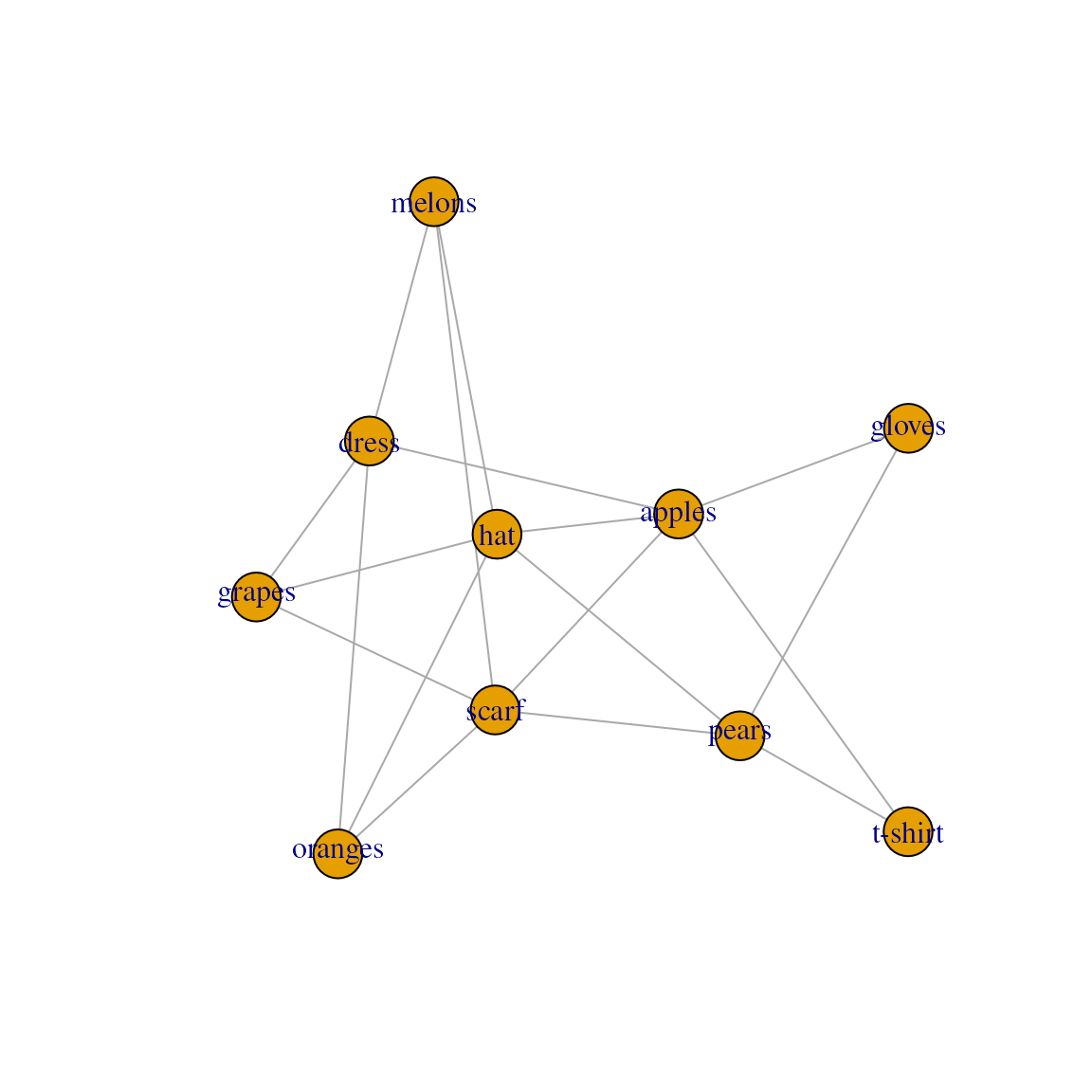
Session Info
sessionInfo()
#> R version 4.6.1 (2026-06-24)
#> Platform: x86_64-pc-linux-gnu
#> Running under: Ubuntu 24.04.4 LTS
#>
#> Matrix products: default
#> BLAS:   /usr/lib/x86_64-linux-gnu/openblas-pthread/libblas.so.3
#> LAPACK: /usr/lib/x86_64-linux-gnu/openblas-pthread/libopenblasp-r0.3.26.so;  LAPACK version 3.12.0
#>
#> locale:
#>  [1] LC_CTYPE=en_US.UTF-8       LC_NUMERIC=C
#>  [3] LC_TIME=en_US.UTF-8        LC_COLLATE=en_US.UTF-8
#>  [5] LC_MONETARY=en_US.UTF-8    LC_MESSAGES=en_US.UTF-8
#>  [7] LC_PAPER=en_US.UTF-8       LC_NAME=C
#>  [9] LC_ADDRESS=C               LC_TELEPHONE=C
#> [11] LC_MEASUREMENT=en_US.UTF-8 LC_IDENTIFICATION=C
#>
#> time zone: UTC
#> tzcode source: system (glibc)
#>
#> attached base packages:
#> [1] stats     graphics  grDevices utils     datasets  methods   base
#>
#> other attached packages:
#> [1] igraph_2.3.3      ragg_1.5.2        systemfonts_1.3.2 ggplot2_4.0.3
#> [5] dplyr_1.2.1       MultiFactor_0.1.2
#>
#> loaded via a namespace (and not attached):
#>  [1] Matrix_1.7-5       gtable_0.3.6       jsonlite_2.0.0     compiler_4.6.1
#>  [5] tidyselect_1.2.1   jquerylib_0.1.4    scales_1.4.0       textshaping_1.0.5
#>  [9] yaml_2.3.12        fastmap_1.2.0      lattice_0.22-9     R6_2.6.1
#> [13] generics_0.1.4     knitr_1.51         htmlwidgets_1.6.4  forcats_1.0.1
#> [17] tibble_3.3.1       desc_1.4.3         RColorBrewer_1.1-3 bslib_0.11.0
#> [21] pillar_1.11.1      rlang_1.3.0        cachem_1.1.0       xfun_0.60
#> [25] fs_2.1.0           sass_0.4.10        S7_0.2.2           otel_0.2.0
#> [29] cli_3.6.6          withr_3.0.3        pkgdown_2.2.1      magrittr_2.0.5
#> [33] digest_0.6.39      grid_4.6.1         lifecycle_1.0.5    vctrs_0.7.3
#> [37] evaluate_1.0.5     glue_1.8.1         farver_2.1.2       rmarkdown_2.31
#> [41] tools_4.6.1        pkgconfig_2.0.3    htmltools_0.5.9